Easy Task for GSOC

Author

Javad Vahdat Atashgah

Task 1 (Easy)

Download the occurrence data of platypus in Australia from the Atlas of Living Australia, and make a map showing the spatial locations of sightings for 2024.

Introduction

The platypus (Ornithorhynchus anatinus), sometimes referred to as the duck-billed platypus, is a semiaquatic, egg-laying mammal endemic to eastern Australia, including Tasmania. The platypus is the sole living representative or monotypic taxon of its family Ornithorhynchidae and genus Ornithorhynchus, though a number of related species appear in the fossil record.

This report shows how to download platypus occurrence data in Australia from the Atlas of Living Australia (ALA) and create a map of sightings from the year 2024.

Start Coding

Install packages if not already installed

install.packages("galah")
install.packages("dplyr")
install.packages("ggplot2")

Load required packages:

library(galah)
library(dplyr)
library(ggplot2)

Set Up ALA Access

Before you can download data, you need to configure the galah package with your email. This email will be used to identify your requests to the ALA servers. You need to sign up in ALA website for using your email address.

galah_config(email = "vahdatjavad@gmail.com") 
# Replace with your email

Search for Platypus Occurrences in 2024

We will query ALA for sightings of Ornithorhynchus anatinus (platypus), limited to Australia and the year 2024.

# Search for the taxon
platypus_taxon <- search_taxa("Ornithorhynchus anatinus")

# Retrieve occurrence data from 2024 using unambiguous scientific name
occ_data <- galah_call() |>
  galah_identify(platypus_taxon) |>
  galah_filter(year == 2024) |>
  galah_select(decimalLatitude, decimalLongitude, year, eventDate, scientificName) |>
  atlas_occurrences()

Filter and Inspect the Data

Make sure the data includes coordinates and relevant variables.

# Drop records with missing coordinates
platypus_2024 <- occ_data |>
  filter(!is.na(decimalLatitude), !is.na(decimalLongitude))

# Peek at the cleaned dataset
head(platypus_2024)

# A tibble: 6 × 5
  decimalLatitude decimalLongitude  year eventDate           scientificName     
            <dbl>            <dbl> <dbl> <dttm>              <chr>              
1           -43.4             147.  2024 2024-07-26 00:00:00 Ornithorhynchus an…
2           -43.2             147.  2024 2024-10-15 00:00:00 Ornithorhynchus an…
3           -43.2             147.  2024 2024-10-15 00:00:00 Ornithorhynchus an…
4           -43.2             147.  2024 2024-12-31 00:00:00 Ornithorhynchus an…
5           -43.2             147.  2024 2024-10-12 00:00:00 Ornithorhynchus an…
6           -43.2             147.  2024 2024-01-08 21:02:13 Ornithorhynchus an…

Saving The Data

save(platypus_2024, file = "../data/platypus_2024.RDA")

This will save the data to a file named platypus_2024.RDA in the data directory. You can load this data in future sessions using:

load(file = "../data/platypus_2024.RDA")

Plotting the Map of Sightings

We’ll create a basic map of platypus sightings across Australia using ggplot2.

ggplot(data = platypus_2024) +
  borders("world", regions = "Australia", fill = "gray95", colour = "gray50") +
  geom_point(aes(x = decimalLongitude, y = decimalLatitude), color = "darkblue", alpha = 0.6, size = 2) +
  coord_fixed(1.3) +
  labs(
    title = "Platypus Sightings in Australia (2024)",
    x = "Longitude",
    y = "Latitude"
  ) +
  theme_minimal()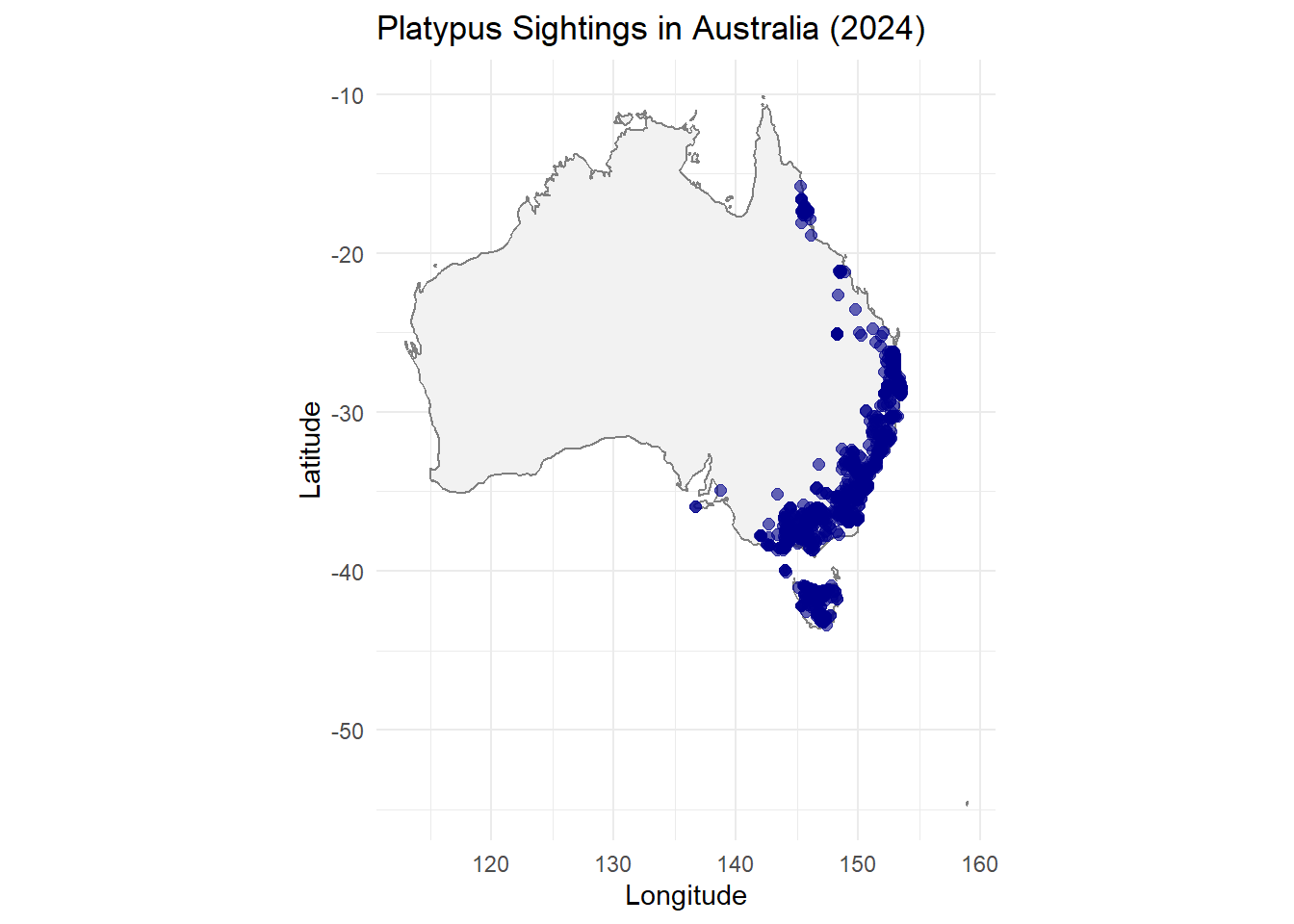

We want to add Month Category for better visualisation

# Install lubridate if not already installed
if (!requireNamespace("lubridate", quietly = TRUE)) {
  install.packages("lubridate")
}

library(dplyr)
library(lubridate)

platypus_2024 <- platypus_2024 %>%
  mutate(
    month_num = month(eventDate),                     
    month_name = month(eventDate, label = TRUE)
  )

library(ggplot2)

ggplot(data = platypus_2024) +
  borders("world", regions = "Australia", fill = "gray95", colour = "gray50") +
  geom_point(aes(x = decimalLongitude, y = decimalLatitude, color = month_name),
             alpha = 0.7, size = 2) +
  coord_fixed(1.3) +
  labs(
    title = "Platypus Sightings in Australia (2024)",
    subtitle = "Colored by Month of Observation",
    x = "Longitude",
    y = "Latitude",
    color = "Month"
  ) +
  theme_minimal()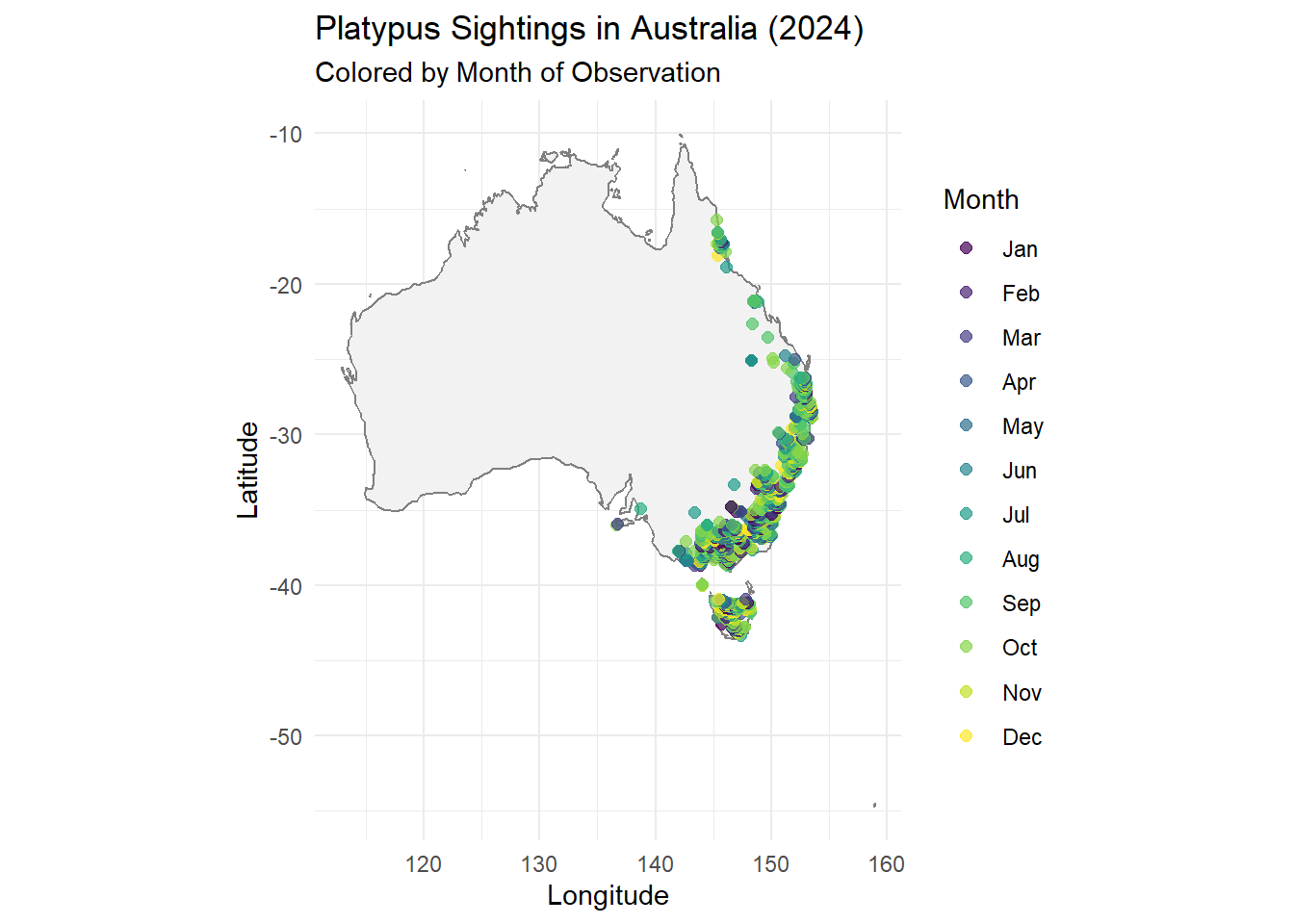

Add season category to data :

platypus_2024 <- platypus_2024 %>%
  mutate(
    season = case_when(
      month_num %in% c(12, 1, 2)  ~ "Summer",
      month_num %in% c(3, 4, 5)   ~ "Autumn",
      month_num %in% c(6, 7, 8)   ~ "Winter",
      month_num %in% c(9, 10, 11) ~ "Spring"
    ),
    season = factor(season, levels = c("Summer", "Autumn", "Winter", "Spring"))
  )

ggplot(data = platypus_2024) +
  borders("world", regions = "Australia", fill = "gray95", colour = "gray70") +
  geom_point(aes(x = decimalLongitude, y = decimalLatitude, color = season),
             alpha = 0.7, size = 2) +
  coord_fixed(1.3) +
  labs(
    title = "Platypus Sightings in Australia (2024)",
    subtitle = "Colored by Season",
    x = "Longitude",
    y = "Latitude",
    color = "Season"
  ) +
  theme_minimal()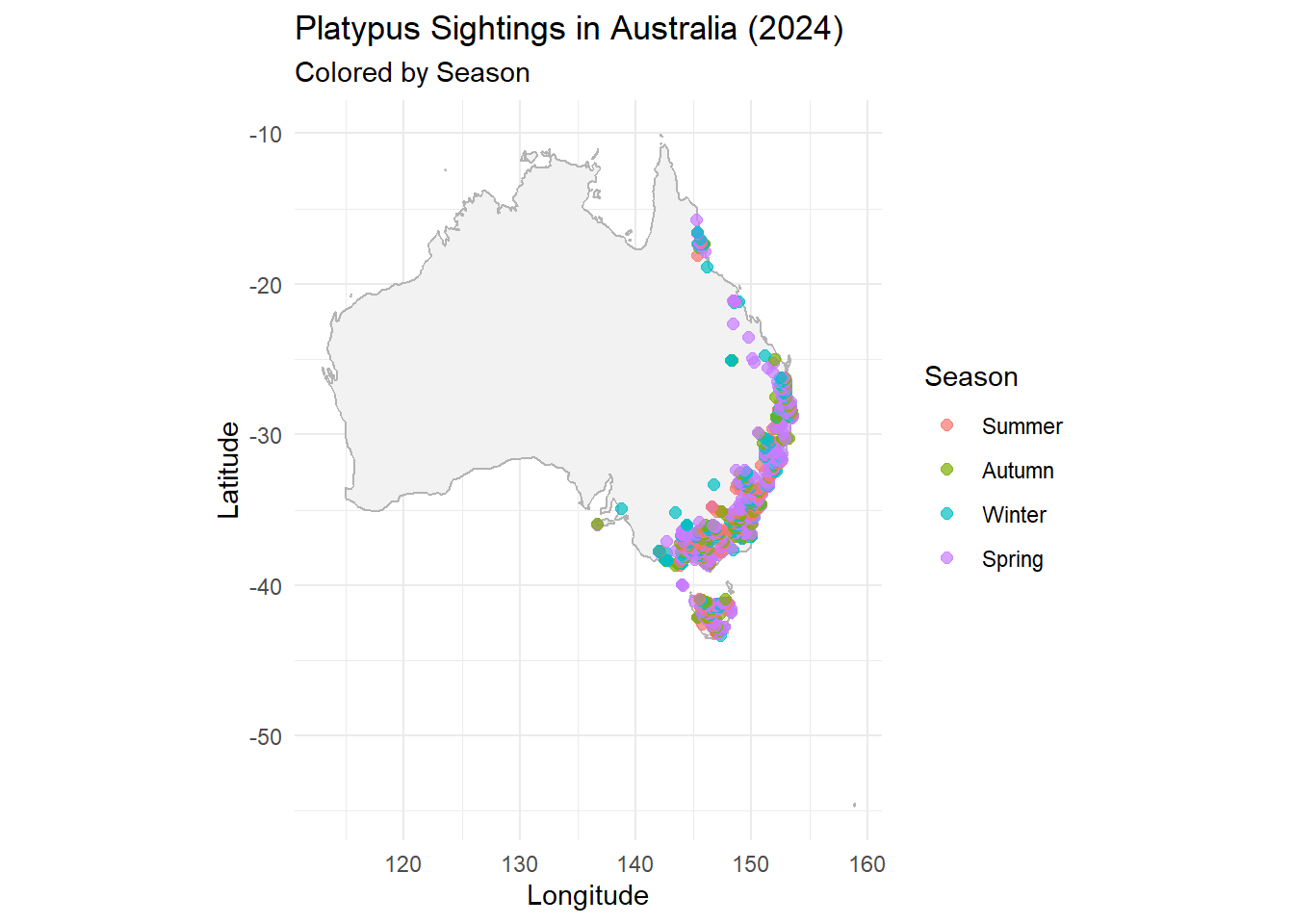

ggplot(data = platypus_2024) +
  borders("world", regions = "Australia", fill = "gray95", colour = "gray70") +
  geom_point(aes(x = decimalLongitude, y = decimalLatitude, color = month_name),
             alpha = 0.6, size = 1.8) +
  coord_fixed(1.3) +
  facet_wrap(~ season) +
  labs(
    title = "Platypus Sightings in 2024: Monthly Patterns within Seasons",
    x = "Longitude",
    y = "Latitude",
    color = "Month"
  ) +
  theme_minimal()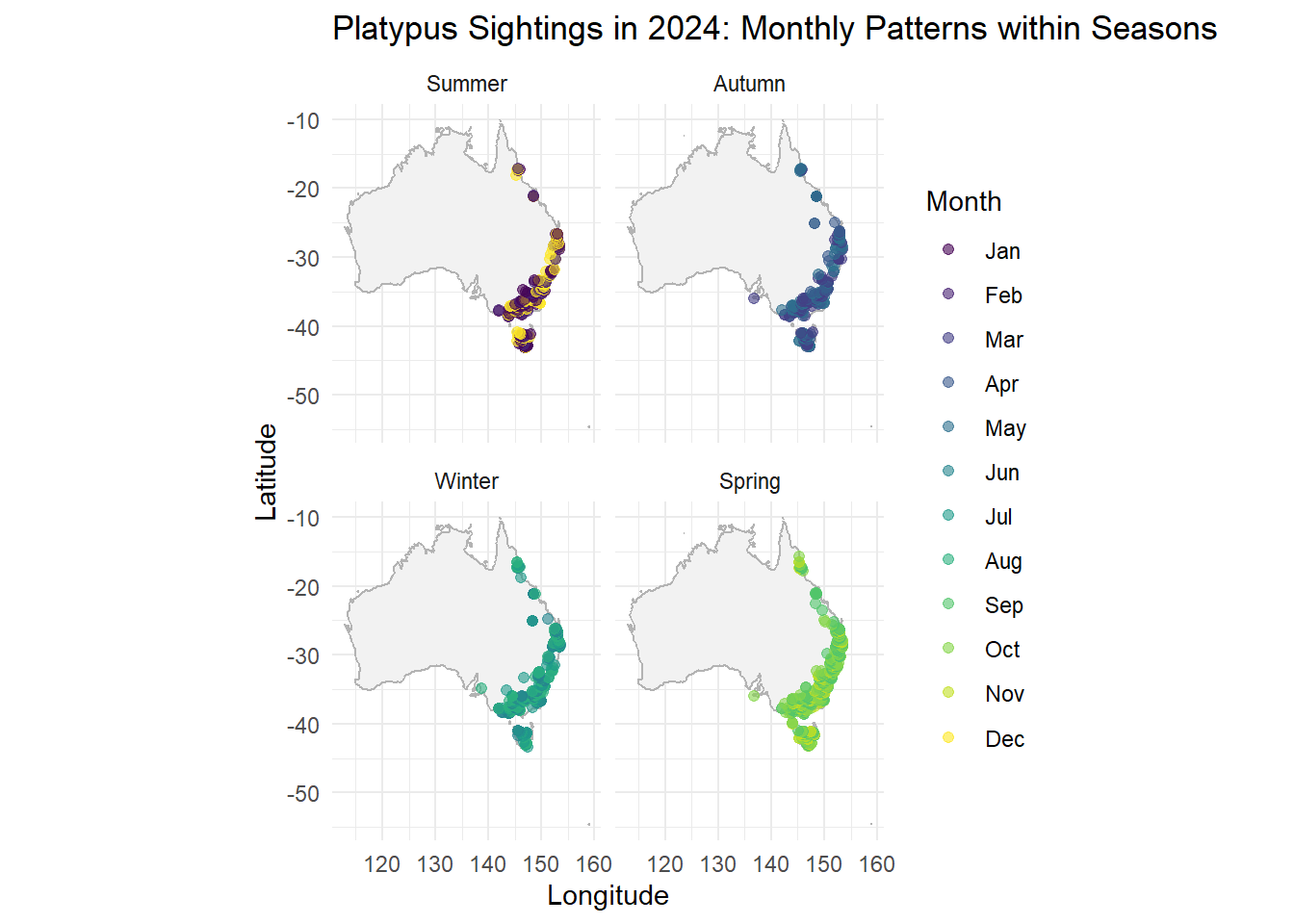

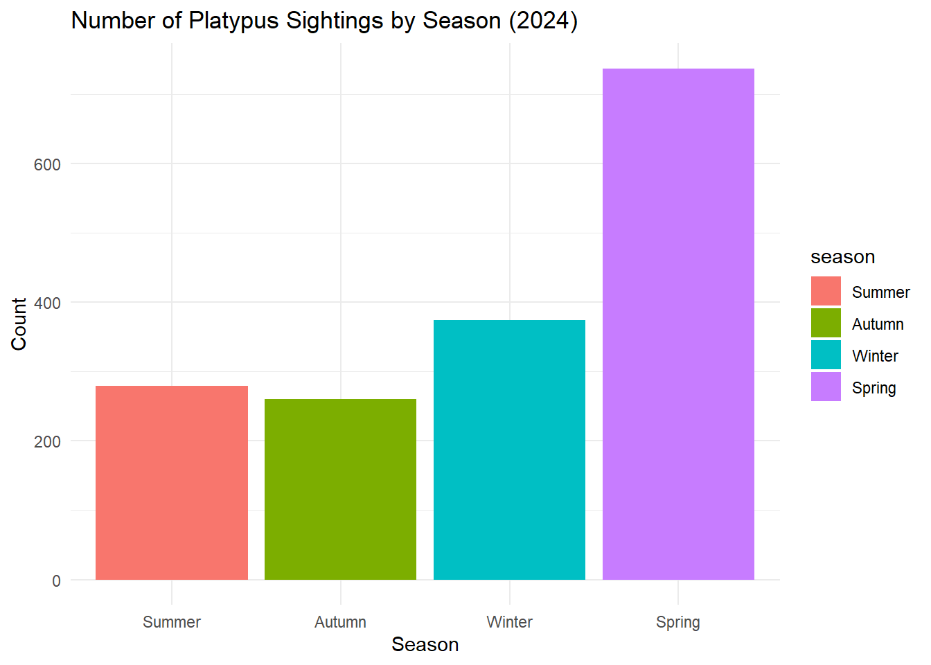
summarize count of sightings per season and make a bar plot to complement the map:

platypus_2024 %>%
  count(season) %>%
  ggplot(aes(x = season, y = n, fill = season)) +
  geom_col() +
  labs(title = "Number of Platypus Sightings by Season (2024)", y = "Count", x = "Season") +
  theme_minimal()