Hard Task for GSOC

Task 3 Hard

Taking the names of tourism locations described in this variable Stopover state/region/SA2 from the data-raw/domestic_trips_2023-10-08.csv write code to geocode the locations with latitude and longitude.

Read and clean the data

load required packages

library(tidyverse)

read the data

raw_data <- read_csv("../../data-raw/domestic_trips_2023-10-08.csv",
                     skip = 9,
                     col_names = FALSE,
                     col_types = cols(X8 = col_skip()),
                     n_max = 248055
                     )

Rename and clean the columns

colnames(raw_data) <- c(
  "Quarter", "Region", "Holiday", "Visiting", "Business", "Other", 
  "Total")
head(raw_data, n = 2)

# A tibble: 2 × 7
  Quarter            Region                Holiday Visiting Business Other Total
  <chr>              <chr>                   <dbl>    <dbl>    <dbl> <dbl> <dbl>
1 March quarter 1998 Baulkham Hills - East       0        0     2.90     0  2.90
2 <NA>               Baulkham Hills (West…       0        0     0        0  0   

Now, fill down the Quarter info:

clean_data <- raw_data %>%
  fill(Quarter, .direction = "down") %>%
  filter(!is.na(Region))  # Remove empty rows
head(clean_data, n = 2)

# A tibble: 2 × 7
  Quarter            Region                Holiday Visiting Business Other Total
  <chr>              <chr>                   <dbl>    <dbl>    <dbl> <dbl> <dbl>
1 March quarter 1998 Baulkham Hills - East       0        0     2.90     0  2.90
2 March quarter 1998 Baulkham Hills (West…       0        0     0        0  0   

Geocode the “Region” column

Now for the geocoding. We have a list of place names — most likely suburb/local area names in Australia. We can use tidygeocoder, which is flexible and integrates with many providers.

Install if needed and then load

if (!requireNamespace("tidygeocoder", quietly = TRUE)) {
  install.packages("tidygeocoder")
}

library(tidygeocoder)

Geocode the unique region names

geocoded_locations <- clean_data %>%
  distinct(Region) %>%
  geocode(
    address = Region,
    method = "osm",   # other methods "arcgis" or "census" 
    lat = latitude,
    long = longitude,
    full_results = FALSE,
    custom_query = list(countrycodes = "AU")
  )
save(geocoded_locations, file = "../data/geocoded_Locations_V1.rds")

load(file = "../data/geocoded_Locations_V1.rds")

use other methods for completing NA records

geocoded_missing <- geocoded_locations |> 
  filter(is.na(latitude) | is.na(longitude)) |>
  geocode(
    address = Region,
    method = "arcgis",    
    lat = latitude,
    long = longitude,
    full_results = FALSE,
    custom_query = list(countrycodes = "AU")
  )
geocoded_missing <- geocoded_missing |> transmute(
  Region = Region, 
  latitude = latitude...4,
  longitude = longitude...5
)
save(geocoded_missing, file = "../data/geocoded_Locations_V2.rds")

load(file = "../data/geocoded_Locations_V2.rds")

Merge results (fill NAs with second try)

geocoded_combined <- geocoded_locations %>%
  rows_update(geocoded_missing, by = "Region") |> 
  filter(!is.na(latitude))

clean_data_with_coords <- clean_data %>%
  left_join(geocoded_combined, by = "Region") |> 
  filter(!is.na(latitude)) |> rename(
    LAT = latitude,
    LON = longitude 
  )

save(clean_data_with_coords, file = "../data/domestic_trips_20231008_geocoded.rda")

clean_data_with_coords |> distinct(Region, .keep_all = T) |> 
ggplot(aes(x = LON, y = LAT)) +
  borders("world", fill = "gray95", colour = "gray50") +
  geom_point(aes(size = Total), color = "darkred", alpha = 0.7) +
  scale_size_continuous(range = c(2, 10)) +
  coord_fixed(1.3) +
  labs(
    title = "Visitor Totals by Region",
    x = "Longitude", y = "Latitude", size = "Total Visitors"
  ) +
  theme_minimal()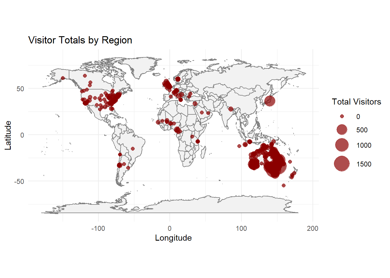

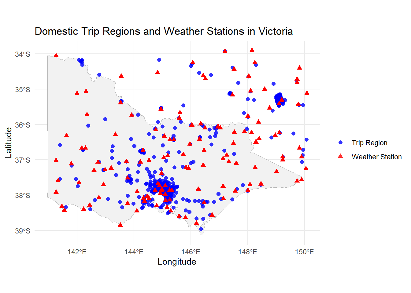
Filter for Victoria

first we filter out domestic data just for Victoria

domestic_trips_VIC <- clean_data_with_coords %>%
  filter(
    LAT >= -39, LAT <= -33.9,
    LON >= 140.9, LON <= 150.1
  )

Then we want to find near-st weather stations to each of this spots.

load Victoria Stations Coordinates

load(file = "../data/vic_stations.RDA")

find the nearest weather station

library(geosphere)

nearest_station_ids <- sapply(1:nrow(domestic_trips_VIC), function(i) {
  dists <- distHaversine(
    cbind(vic_stations$LON, vic_stations$LAT),
    c(domestic_trips_VIC$LON[i], domestic_trips_VIC$LAT[i])
  )
  vic_stations$STNID[which.min(dists)]
})

Add nearest station ID to domestic_trips_VIC

domestic_trips_VIC$STNID <- nearest_station_ids

save data GC geocoded STNID nearest station ids

save(domestic_trips_VIC, file = "../data/domestic_trips_VIC_GC_STNID.rda")

library(ozmaps)

# Prepare region points
region_points <- domestic_trips_VIC %>%
  distinct(Region, LAT, LON) %>%
  mutate(Type = "Trip Region")

# Prepare station points
station_points <- vic_stations %>%
  rename(LAT = LAT, LON = LON) %>%
  mutate(Type = "Weather Station")

# Combine both for legend
combined_points <- bind_rows(region_points, station_points)

# Plot with legend
ggplot() +
  geom_sf(data = ozmaps::ozmap_states %>% filter(NAME == "Victoria"), fill = "gray95", color = "gray70") +
  geom_point(data = combined_points, aes(x = LON, y = LAT, color = Type, shape = Type), size = 2, alpha = 0.8) +
  scale_color_manual(values = c("Trip Region" = "blue", "Weather Station" = "red")) +
  scale_shape_manual(values = c("Trip Region" = 16, "Weather Station" = 17)) +  # dot and triangle
  labs(
    title = "Domestic Trip Regions and Weather Stations in Victoria",
    x = "Longitude", y = "Latitude",
    color = "", shape = ""
  ) +
  coord_sf() +
  theme_minimal() +
  theme(legend.position = "right")